In the past decade, the development of high-throughput methods for genomic sequencing (next-generation sequencing: NGS) have revolutionized how many geneticists collect data. It is now possible to produce so much data so rapidly that simply storing and processing the data poses great challenges . The Nekrutenko and Taylor review doesn’t even discuss the new challenges that face population geneticists and evolutionary biologists as they start to take advantage of those tools, nor did it discuss the promise these data hold for providing new insight into long-standing questions, but the challenges and the promise are at least as great as those they do describe.
To some extent the most important opportunity provided by NGS sequencing is simply that we now have a lot more data to answer the same questions. For example, using a technique like RAD sequencing or genotyping-by-sequencing (GBS: ), it is now possible to identify thousands of polymorphic SNP markers in non-model organisms, even if you don’t have a reference genome available. As we’ve seen several times this semester, the variance associated with drift is enormous. Many SNPs identified through RAD-Seq or GBS are likely to be independently inherited. Thus, the amount and pattern of variation at each locus will represent an independent sample from the underlying evolutionary process. As a result, we should be able to get much better estimates of fundamental parameters like \(\theta=4N_e\mu\), \(M=4N_em\), and \(R=4N_er\) and to have much greater power to discriminate among different evolutionary scenarios. Willing et al. , for example, present simulations suggesting that accurate estimates of \(F_{ST}\) are possible with sample sizes as small as 4–6 individuals per population, so long as the number of markers used for inference is greater than 1000.
I won’t review the chemistry used for next-generation sequencing. It changes very rapidly, and I can’t keep up with it. Suffice it to say that 454 Life Sciences, Illumina, PacBio, and probably other companies I don’t know about each have different approaches to very high throughput DNA sequencing. What they all have in common is that the whole genome is broken into small fragments and sequnced and that a single run through the machine produces an enormous amount of data, 134-6000 Gb and up to 20 billion readsfrom a NovaSeq 600 for example (https://www.illumina.com/systems/sequencing-platforms/comparison-tool.html; accessed 30 December 2018).1
Baird et al. introduced RAD almost 10 years ago. One of its great attraction for evolutionary geneticists is that RAD-seq can be used in any organism from which you can extract DNA and the laboratory manipulations are relatively straightforward.
Digest genomic DNA from each individual with a restriction enzyme, and ligate an adapter to the resulting fragments. The adapter includes a forward amplification primer, a sequencing primer and a “barcode” used to identify the individual from which the DNA was extracted.
Pool the individually barcoded samples (“normalizing” the mixture so that roughly equal amounts of DNA from each individual are present) shear them and select those of a size appropriate for the sequencing platform you are using.
Ligate a second adapter to the sample, where the second adapter is the reverse complement of the reverse amplification primer.
PCR amplification will enrich only DNA fragments having both the forward and reverse amplification primer.
The resulting library consists of sequences within a relatively small distance from restriction sites.
Genotyping-by-sequencing (GBS) is a similar approach.
Digest genomic DNA with a restriction enzyme and ligate two adapters to the genomic fragments. One adapter contains a barcode and the other does not.
Pool the samples.
PCR amplify and sequence. Not all ligated fragments will be sequenced because some will contain only one adapter and some fragments will be too long for the NGS platform.
Once an investigator has her sequenced fragments back, she can either map the fragments back to a reference genome or she can assemble the fragments into orthologous sequences de novo. I’m not going to discuss either of those processes, but you can imagine that there’s a lot of bioinformatic processing going on. What I want to focus on is what you do with the data and how you interpret it.
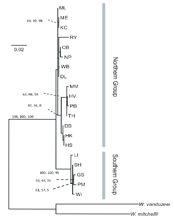
The American pitcher plant mosquito Wyeomyia smithii has been extensively studied for many years. It’s a model organism for ecology, but its genome has not been sequenced. An analysis of COI from 20 populatins and two outgroups produced the set of relationships you see in Figure 1 . As you can see, this analysis allows us to distinguish a northern group of populations from a southern group of populations, but it doesn’t provide us any reliable insight into finer scale relationships.

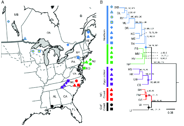
Using the same set of samples, the authors used RAD sequencing to identify 3741 SNPs. That’s more than 20 times the number of variable sites found in COI, 167. Not surprisingly, the large number of additional sites allowed the authors to produce a much more highly resolved phylogeny (Figure 2). With this phylogeny it’s easy to see that southern populations are divided into two distinct groups, those from North Carolina and those from the Gulf Coast. Similarly, the northern group of populations is subdivided into those from the Appalachians in North Carolina, those from the mid-Atlantic coast, and those from further north. The glacial history of North America means that both the mid-Atlantic populations and the populations farther north must have been derived from one or more southern populations after the height of the last glaciation. Given the phylogenetic relationships recovered here, it seems clear that they are most closely related to populations in the Appalachians of North Carolina.
That’s the promise of NGS for population genetics. What are the challenges? Funny you should ask.
Beyond the simple challenge of dealing with all of the short DNA fragments that emerge from high-throughput sequencing, there are at least two challenges that don’t arise with data obtained in more traditional ways.
Most studies involve “shotgun” sequencing of entire genomes. In large diploid genomes, this leads to variable coverage. At sites where coverage is low, there’s a good chance that all of the reads will be derived from only one of the two chromosomes present, and a heterozygous individual will be scored as homozygous. “Well,” you might say, “let’s just throw away all of the sites that don’t have at least 8\(\times\) coverage.”3 That would work, but you would also be throwing out a lot of potentially valuable information.4 It seems better to develop an approach that lets us use all of the data we collect.
Sequencing errors are more common with high-throughput methods than with traditional methods, and since so much data is produced, it’s not feasible to go back and resequence apparent polymorphisms to see if they reflect sequencing error rather than real differences. Quality scores can be used, but they only reflect the quality of the reads from the sequencing reaction, not errors that might be introduced during sample preparation. Again, we might focus on high-coverage sites and ignore “polymorphisms” associated with single reads, but we’d be throwing away a lot of information.5
A better approach than setting arbitrary thresholds and throwing away data is to develop an explicit model of how errors can arise during sequencing and to use that model to interpret the data we’ve collected. That’s precisely the approach that Lynch adopts. Here’s how it works assuming that we have a sample from a single, diploid individual:
Any particular site will have a sequence profile, \((n_1, n_2, n_3, n_4)\), corresponding to the number of times an A, C, G, or T was observed. \(n=n_1+n_2+n_3+n_4\) is the depth of coverage for that site.
Let \(\epsilon\) be the probability of a sequencing error at any site, and assume that all errors are equiprobable, e.g., there’s no tendency for an A to be miscalled as a C rather than a T when it’s miscalled.6
If the site in question were homozygous A, the probability of getting our observed sequence profile is: \[P(n_1,n_2,n_3,n_4|\mbox{homozygous A},\epsilon) = {n \choose n_1}(1-\epsilon)^{n_1}\epsilon^{n-n_1} \quad .\] A similar relationship holds if the site were homozygous C, G, or T. Thus, we can calculate the probability of our data if it were homozygous as7 \[P(n_1,n_2,n_3,n_4|\mbox{homozygous},\epsilon) = \sum_{i=1}^4 \left(\frac{p_i^2}{\sum_{j=1}^4p_j^2}\right) {n \choose n_i}(1-\epsilon)^{n_i}\epsilon^{n-n_i} \quad .\]
If the site in question were heterozygous, the probability of getting our observed sequence profile is a bit more complicated. Let \(k_1\) be the number of reads from the first chromosome and \(k_2\) be the number of reads from the second chromosome (\(n=k_1+k_2\)). Then \[\begin{aligned} P(k_1,k_2) &=& {n \choose k_1}\left(\frac{1}{2}\right)^{k_1} \left(\frac{1}{2}\right)^{k_2} \\ &=& {n \choose k_1}\left(\frac{1}{2}\right)^n \quad .\end{aligned}\] Now consider the ordered genotype \(x_ix_j\), where \(x_i\) refers to the nucleotide on the first chromosome and \(x_j\) refers to the nucleotide on the second chromosome. The probability of getting our observed sequence profile from this genotype given that we have \(k_1\) reads from the first chromosome and \(k_2\) reads from the second is: \[\begin{aligned} P(n_1,n_2,n_3,n_4|x_i,x_j,k_1,k_2) &=& \sum_{l=1}^4\sum_{m=0}^{k_1}{k_1 \choose m}(1-\delta_{il})^m\delta_{il}^{k_1-m} {k_2 \choose n_i-m}(1-\delta_{jl})^{n_1-m}\delta_{jl}^{k_2-(n_1-m)} \quad ,\end{aligned}\] where \[\delta_{il} = \left\{\begin{array}{ll} 1-\epsilon & \mbox{if } i = l \\ \epsilon & \mbox{if } i \ne l \quad . \end{array} \right.\] We can use Bayes’ Theorem8 to get \[P(n_1,n_2,n_3,n_4|x_i,x_j,\epsilon) = P(n_1,n_2,n_3,n_4|x_i,x_j,k_1,k_2,\epsilon)P(k_1,k_2) \quad ,\] and with that in hand we can get \[P(n_1,n_2,n_3,n_4|\mbox{heterozygous},\epsilon) = \sum_{i=1}^4\sum_{j\ne i} \left(\frac{x_ix_j}{1-{\sum_{l=1}^4p_l^2}}\right) P(n_1,n_2,n_3,n_4|x_i,x_j,\epsilon)\]
Let \(\pi\) be the probability that any site is heterozygous. Then the probability of getting our data is: \[P(n_1,n_2,n_3,n_4|\pi,\epsilon) = \pi P(n_1,n_2,n_3,n_4|\mbox{heterozygous},\epsilon) + (1-\pi)P(n_1,n_2,n_3,n_4|\mbox{homozygous},\epsilon) \quad .\]
What we’ve just calculated is the probability of the configuration we observed at a particular site. The probability of our data is just the product of this probability across all of the sites in our sample: \[P(\mbox{data}|\pi,\epsilon) = \prod_{s=1}^S P(n_1^{(s)},n_2^{(s)},n_3^{(s)},n_4^{(s)}|\pi,\epsilon) \quad ,\] where the superscript \((s)\) is used to index each site in the data.
What we now have is the likelihood of the data in terms of \(\epsilon\), which isn’t very interesting since it’s just the average sequencing error rate in our sample, and \(\pi\), which is interesting, because it’s the genome-wide nucleotide diversity. Now we “simply” maximize that likelihood, and we have maximum-likelihood estimates of both parameters. Alternatively, we could supply priors for \(\epsilon\) and \(\pi\) and use MCMC to get Bayesian estimates of \(\epsilon\) and \(\pi\).
Notice that this genome-wide estimate of nucleotide diversity is obtained from a sample derived from a single diploid individual. Lynch develops similar methods for estimating gametic disequilibrium as a function of genetic distance for a sample from a single diploid individual. He also extends that method to samples from a pair of individuals, and he describes how to estimate mutation rates by comparing sequences derived from individuals in mutation accumulation lines with consensus sequences.9
Haubold et al. describe a program implementing these methods. Recall that under the infinite sites model of mutation \(\pi = 4N_e\mu\). They analyzed data sets from the sea squirt Ciona intestinalis and the water flea Daphnia pulex (Table 1). Notice that the sequencing error rate in D. pulex is indistinguishable from the nucleotide diversity.
| Taxon | \(4N_e\mu\) | \(4N_e\mu\) (low coverage) | \(\epsilon\) |
|---|---|---|---|
| Cionia intestinalis | 0.0111 | 0.012 | 0.00113 |
| Daphnia pulex | 0.0011 | 0.0012 | 0.00121 |
What we’ve discussed so far gets us estimates of some population parameters (\(4N_e\mu\), \(4N_er\)), but they’re derived from the sequences in a single diploid individual. That’s not much of a population sample, and it certainly doesn’t tell us anything about how different populations are from one another. Gompert and Buerkle describe an approach to estimate statistics very similar to \(\Phi_{ST}\) from AMOVA. Since they take a Bayesian approach to developing their estimates, they refer to approach as BAMOVA, Bayesian models for analysis of molecular variance. They propose several related models.
NGS-individual model: This model assumes that sequencing errors are negligible.11 Under this model, the only trick is that we may or may not pick up both sequences from a heterozygote. The probability of not seeing both sequences in a heterozygote is related to the depth of coverage.
NGS-population model: In some NGS experiments, investigators pool all of the samples from a population into a single sample. Again, Gompert and Buerkle assume that sequencing errors are negligible. Here we assume that the number of reads for one of two alleles at a particular SNP site in a sample is related to the underlying allele frequency at that site. Roughly speaking, the likelihood of the data at that site is then \[P(x_i|p_i,n_i, k_i) = {n_i \choose k_i}p_i^{k_i}(1-p_{i})^{n-k_i} \quad ,\] where \(p_i\) is the allele frequency at this site, \(n_i\) is the sample size, and \(k_i\) is the count of one of the alleles in the sample. The likelihood of the data is just the product across the site-specific likelihoods.12
Then, as we did way back when we used a Bayesian appraach to estimate \(F_{ST}\) , we put a prior on the \(p_i\) and the parameters of this prior are defined in terms of \(\Phi_{ST}\) (among other things).13 They also propose a method for detecting SNP loci14 that have unusually large or small values of \(\Phi_{ST}\).
Gompert and Buerkle used data derived from two different human population data sets:
316 fully sequenced genes in an African population and a population with European ancestry. With these data, they didn’t have to worry about the sequencing errors that their model neglects and they could simulate pooled samples allowing them to compare estimates derived from pooled versus individual-level data.
12,649 haplotype regions and 11,866 genes derived from 597 individuals across 33 widely distributed human populations.
In analysis of the first data set, they estimated \(\Phi_{ST}=0.08\). Three loci were identified as having unusually high values of \(\Phi_{ST}\).
HSD11B2: \(\Phi_{ST}=0.32 (0.16,0.48)\). Variants at this locus are associated with an inherited form of high blood pressure and renal disease. A microsatellite in an intron of this locus is weakly associated with type 1 diabetes.
FOXA2: \(\Phi_{ST}=0.32 (0.12,0.51)\). This gene is involved in reguation of insulin sensitivity.
POLG2: \(\Phi_{ST}=0.33 (0.18,0.48)\). This locus was identified as a target of selection in another study.
In analysis of the 33-population data set, they found similar values of \(\Phi_{ST}\) on each chromosome, ranging from 0.083 (0.075, 0.091) on chromosome 22 to 0.11 (0.10, 0.12) on chromosome 16. \(\Phi_{ST}\) for the X chromosome was marginally higher: 0.14 (0.13,0.15). They detected 569 outlier loci, 518 were high outliers and 51 were low outliers. Several of the loci they detected as outliers had been previously identified as targets of selection. The loci they identified as candidates for balancing selection have not been suggested before as targets of such selection.
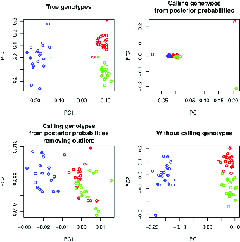
In addition to \(F_{ST}\) we saw that a principal components analysis of genetic data might sometimes be useful. Fumagalli et al. develop a method for PCA that, like Lynch’s method for estimating nucleotide diversity, uses all of the information available in NGS data rather than imposing an artificial threshold for calling genotypes. They calculate the pairwise entries of the covariance matrix by integrating across the genotype probabiity at each site as part of the calculation and weighting the contribution of each site to the analysis by the probability that it is variable.15 As shown in Figure 3 this approach to PCA recovers the structure much better than approaches that simply call genotypes at each locus, whether or not outliers are excluded. The authors also describe approaches to estimating \(F_{ST}\) that take account of the characteristics of NGS data. Their software (ANGSD: http://popgen.dk/wiki/index.php/ANGSD) implements these and other useful statistical analysis tools for next-generation sequencing data, including Tajima’s D. They also provide NgsAdmix for Structure-like analyses of NGS data (http://www.popgen.dk/software/index.php/NgsAdmix).
As we’ve seen several times in this course, the amount of genetic data available on humans is vastly greater than what is available for any other organism. As a result, it’s possible to use these data to gain unusually deep insight into the recent history of many human populations. Today’s example comes from Great Britain, courtesy of a very large consortium
2039 individuals with four grandparents born within 80km of one another, effectively studying alleles sampled from grandparents (ca. 1885).
6209 samples from 10 countries in continental Europe.
Autosomal SNPs genotyped in both samples (ca. 500K).
Very little evidence of population structure within British sample
Average pairwise \(F_{ST}\): 0.0007
Maximum pairwise \(F_{ST}\): 0.003
Individual assignment analysis of genotypes used fineSTRUCTURE, which uses the same principle as STRUCTURE but models the correlations among SNPs resulting from gametic disequilibrium, rather than treating each locus as being independently inherited. The analysis is on haplotypes rather than on alleles. In addition, it clusters populations hierarchically (Figure 4
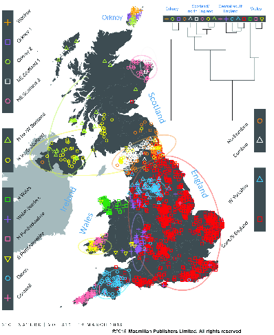
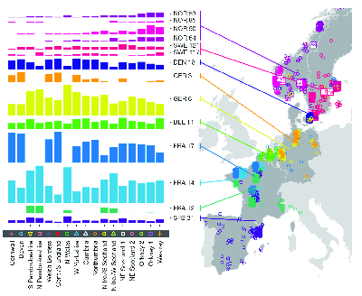
fineSTRUCTURE analysis of genotypes from Great Britain (from ).Analysis of the European data identifies 52 groups. The authors used Chromopainter to construct each of the haplotypes detected in their sample of 2039 individuals from the UK as a mosaic of haplotypes derived from those found in their sample of 6209 individuals from continental Europe. Since they know (a) the UK cluster to which each UK individual belongs and (b) the European group from which each individual contributing to the UK mosaic belongs they can estimate (c) the proportion of ancestry for each UK cluster derived from each European group. The results are shown in Figure 5.
These notes are licensed under the Creative Commons Attribution License. To view a copy of this license, visit https://creativecommons.org/licenses/by/4.0/ or send a letter to Creative Commons, 559 Nathan Abbott Way, Stanford, California 94305, USA.
In NGS applications for phylogeny, a strategy of targeted enrichment is often used. In this approach, pre-identified parts of the genome are “baited” using primers and those parts of the genome are enriched through PCR before the sequencing library is constructed . By the way, when I taught this course two years ago the Illumina HiSeq X Ten produced the most data from a single run, up to 1800 Gb and 3-6 billion reads. That means the volume of sequence you can produce in a single run has tripled in two years.↩︎
This section draws heavily on ↩︎
If both chromosomes have an equal probability of being sequenced, the probability that one of them is missed with 8\(\times\) coverage is \((1/2)^8 = 1/256\).↩︎
It’s valuable information, providing you know how to deal with in properly.↩︎
To be honest, though, we did ignore a lot of data in the analysis of GBS data from Protea repens that you may remember from earlier this semester.↩︎
It wouldn’t be hard, conceptually, to allow different nucleotides to have different error rates, e.g., \(\epsilon_A\), \(\epsilon_C\), \(\epsilon_G\), \(\epsilon_T\), but the notation would get really complicated, so we won’t bother trying to show how differential error rates can be accommodated.↩︎
This expression looks a little different from the one in , but I’m pretty sure it’s equivalent.↩︎
Ask me for details if you’re interested.↩︎
Mutation accumulation lines are lines propagated through several (sometimes up to hundreds) of generations in which population sizes are repeatedly reduced to one or a few individuals, allowing drift to dominate the dynamics and alleles to “accumulate” with little regard to their fitness effects.↩︎
This section depends heavily on ↩︎
Or that they’ve already been corrected. We don’t care how they might have been corrected. We care only that we can assume that the reads we get from a sequencing run faithfully reflect the sequences present on each of the chromosomes.↩︎
The actual model they use is a bit more complicated than this, but the principles are the same.↩︎
Again, the actual model is a bit more complicated than what I’m describing here, but the principle is the same.↩︎
Or sets of SNP loci that are parts of a single contig.↩︎
See for details.↩︎